3D Space Visualization

space_profile visualizes 3D vector fields (e.g. displacement fields) as arrows, powered by PyVista. space_animation plays time-dependent vector fields in an interactive PyVista window.

Installation

pip install ferrodispcalc[vis]

Quick Start

from ase.io import read
from ferrodispcalc.compute import calculate_displacement
from ferrodispcalc.neighborlist import build_neighbor_list
from ferrodispcalc.vis import grid_data, space_profile

atoms = read("structure.vasp")
nl = build_neighbor_list(atoms, ["Pb"], ["O"], 4, 12, False)
disp = calculate_displacement(atoms, nl)
d_grid, coord = grid_data(atoms, disp, ["Pb"],
                           target_size=[40, 20, 11],
                           return_coord=True)

# Grid mode (recommended -- supports gradient coloring)
space_profile(d_grid, color_by="dz", cmap="coolwarm", factor=25.0)

# Or point mode
pts = coord.reshape(-1, 3)
vecs = d_grid.reshape(-1, 3)
space_profile(vecs, coord=pts, color_by="magnitude")

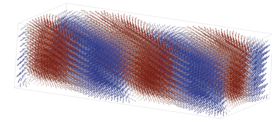
../_images/space_profile_example.png — Example output of `space_profile` with `color_by="dz"`.

Input Modes

space_profile accepts two data layouts:

Grid mode – data has shape (nx, ny, nz, 3). Coordinates are generated automatically from grid indices; the coord argument is ignored.
Point mode – data has shape (npoint, 3). You must also pass coord with the same shape.

Coloring (`color_by`)

Controls how arrows are colored:

'magnitude' – vector norm
'dx' / 'dy' / 'dz' – single component value
'all' – RGB mapping (each component normalized to [0, 1])
'gradient' – gradient field magnitude (grid mode only)

cmap sets the matplotlib colormap (default "coolwarm"; ignored when color_by="all"). clim overrides the colorbar range, e.g. clim=(-0.2, 0.2).

Region Selection (`select`)

Display a sub-region by filtering in fractional coordinates. In grid mode, fractions are derived from grid indices automatically. In point mode, you must also pass the cell parameter (the 3x3 lattice matrix):

# Grid mode -- no cell needed
space_profile(d_grid, color_by="dz",
              select={"x": [0.5, 1.0], "y": None, "z": None})

# Point mode -- cell required
import numpy as np
cell = np.array(atoms.cell)
space_profile(vecs, coord=pts, color_by="dz",
              select={"x": [0.5, 1.0], "y": None, "z": None},
              cell=cell)

Each key ('x', 'y', 'z') maps to a [lo, hi] range or None (no filtering on that axis).

Display Options

factor – arrow scale factor (default 25.0)
projection – "ortho" (default) or "persp"
show_bounding_box – draw a wireframe box around the full point cloud (default True)
show_axes – show the XYZ orientation widget (default True)

Animation

Use space_animation for time-dependent 3D vector fields. Grid-mode animations use (nframe, nx, ny, nz, 3) data. Point-mode animations use (nframe, npoint, 3) data with a matching coord array.

from ferrodispcalc.vis import space_animation

# disp_grid has shape (nframe, nx, ny, nz, 3)
space_animation(
    disp_grid,
    color_by="dz",
    cmap="coolwarm",
    factor=10.0,
    stride=(2, 1, 1),
    frame_step=2,
    fps=20,
)

The animation window includes a frame slider. Press space to pause or resume playback, and use the left/right arrow keys to step through displayed frames. For large datasets, use stride for spatial down-sampling and frame_step or frame_indices for temporal down-sampling.

Custom Plotter

Pass an existing pv.Plotter to overlay multiple visualizations or customize the scene. When a plotter is provided, space_profile adds meshes to it but does not call show(), so you retain full control:

import pyvista as pv

pl = pv.Plotter()
space_profile(d_grid, color_by="dz", plotter=pl)
pl.show()

API Reference

ferrodispcalc.vis.space_plot.space_profile(data: np.ndarray, coord: np.ndarray | None = None, *, color_by: str = 'dz', cmap: str = 'coolwarm', factor: float = 25.0, projection: str = 'ortho', clim: tuple[float, float] | None = None, select: dict | None = None, cell: np.ndarray | None = None, title: str = '3D Vector Field', show_bounding_box: bool = True, show_axes: bool = True, plotter: pv.Plotter | None = None) → pv.Plotter[source]

Plot a 3D vector field using PyVista.

Two input modes are supported:

Grid mode – data has shape (nx, ny, nz, 3). Coordinates are generated automatically from grid indices and coord is ignored.
Point mode – data has shape (npoint, 3) and coord (also (npoint, 3)) must be provided.

Parameters:

data (np.ndarray) – Vector data. (nx, ny, nz, 3) for grid mode or (npoint, 3) for point mode.
coord (np.ndarray or None) – Cartesian coordinates (npoint, 3). Required for point mode, ignored for grid mode.
color_by (str) – Coloring strategy: 'magnitude', 'dx', 'dy', 'dz', 'all' (RGB from components), or 'gradient' (grid mode only).
cmap (str) – Matplotlib colormap name (ignored when color_by=’all’).
factor (float) – Arrow scale factor passed to pv.PolyData.glyph.
projection (str) – 'ortho' for parallel projection, 'persp' for perspective.
clim (tuple or None) – Colorbar range (vmin, vmax). None for automatic.
select (dict or None) – Region filter in fractional coordinates. Keys are 'x', 'y', 'z'; values are [lo, hi] or None (no filter). In grid mode fractions are computed from grid indices; in point mode cell is required.
cell (np.ndarray or None) – (3, 3) lattice matrix (rows = lattice vectors). Only needed when select is used in point mode.
title (str) – Window title.
show_bounding_box (bool) – Draw a wireframe box around the full point cloud.
show_axes (bool) – Show orientation axes widget.
plotter (pv.Plotter or None) – Reuse an existing plotter. A new one is created when None.

Returns:

The plotter instance (already shown).

Return type:

pv.Plotter

ferrodispcalc.vis.space_plot.space_animation(data: np.ndarray, coord: np.ndarray | None = None, *, color_by: str = 'dz', cmap: str = 'coolwarm', factor: float = 25.0, projection: str = 'ortho', clim: tuple[float, float] | None=None, select: dict | None = None, cell: np.ndarray | None = None, title: str = '3D Vector Field Animation', show_bounding_box: bool = True, show_axes: bool = True, show_slider: bool = True, show_frame_text: bool = True, plotter: pv.Plotter | None = None, stride: int | Sequence[int] = 1, frame_indices: Sequence[int] | slice | None = None, frame_step: int = 1, fps: float = 20.0, autoplay: bool = True, loop: bool = True, dtype: type | str | np.dtype = <class 'numpy.float32'>) → pv.Plotter[source]

Play a 3-D vector-field animation in a PyVista window.

Two time-dependent input modes are supported:

Grid mode - data has shape (nframe, nx, ny, nz, 3). Coordinates are generated automatically from grid indices and coord is ignored.
Point mode - data has shape (nframe, npoint, 3) and coord has shape (npoint, 3).

The scene is created once and updated in-place as frames advance. A slider widget is shown by default for direct frame selection. Keyboard shortcuts are available when more than one frame is selected: space toggles playback, and the left/right arrow keys step backward/forward by one displayed frame.