Example: PTO-STO Superlattice Polarization

This example computes and visualizes local polarization in a PbTiO₃/SrTiO₃ (PTO/STO) superlattice. For core concepts, see Introduction to ferrodispcalc.

Complete Script

from ase.io import read
from ferrodispcalc.neighborlist import build_neighbor_list
from ferrodispcalc.compute import calculate_polarization
from ferrodispcalc.vis import grid_data, plane_profile

atoms = read("stru.traj")

# Build neighbor lists
nl_bo = build_neighbor_list(atoms, ["Ti"], ["O"], cutoff=4, neighbor_num=6)
nl_ba = build_neighbor_list(atoms, ["Ti"], ["Pb", "Sr"], cutoff=4, neighbor_num=8)

# Averaged Born effective charges
z_a = 0.5 * (3.45 + 2.56)
z_b = 0.5 * (5.21 + 7.40)
z_o = -(z_a + z_b) / 3
bec = {"Pb": z_a, "Sr": z_a, "Ti": z_b, "O": z_o}

# Calculate and visualize
P = calculate_polarization(atoms, nl_ba, nl_bo, bec)
P_grid = grid_data(atoms, P, element=["Ti"], target_size=(40, 20, 20))
plane_profile(P_grid, save_dir="profile", select={"x": [0]})

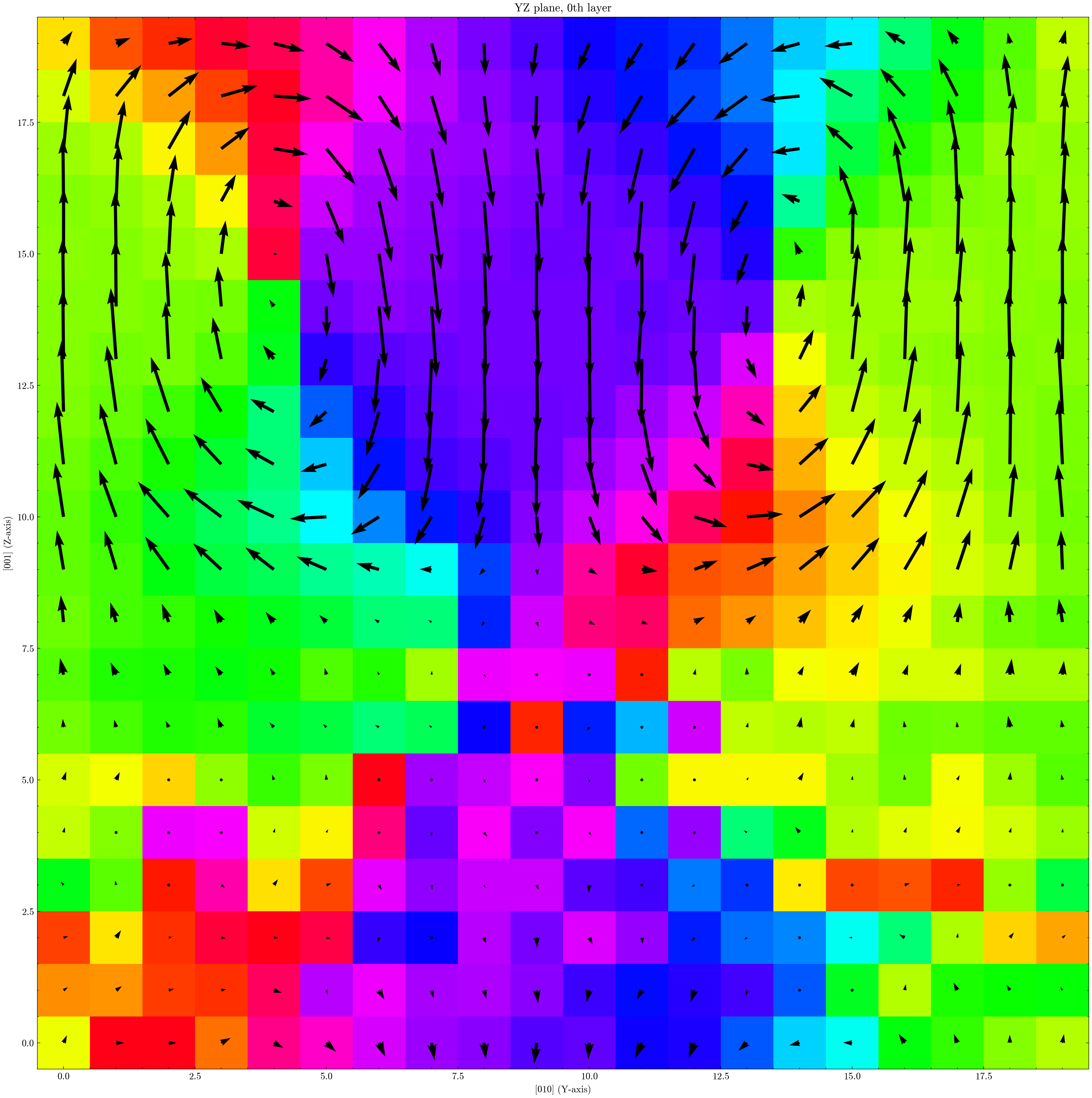
../_images/superlattice_YZ_0.png — Local polarization on the YZ plane (x = 0) of a PTO/STO superlattice.

Step-by-Step Breakdown

Read the Structure

from ase.io import read

atoms = read("stru.traj")

Build Neighbor Lists

In a superlattice, the A-site is occupied by mixed species (Pb and Sr). The key difference from a pure perovskite: pass both species in the neighbor element list.

from ferrodispcalc.neighborlist import build_neighbor_list

# B-O: 6 neighbors (octahedral coordination)
nl_bo = build_neighbor_list(atoms, ["Ti"], ["O"], cutoff=4, neighbor_num=6)

# B-A: 8 neighbors — ["Pb", "Sr"] covers both A-site species
nl_ba = build_neighbor_list(atoms, ["Ti"], ["Pb", "Sr"], cutoff=4, neighbor_num=8)

Calculate Polarization

For a 50/50 PTO-STO superlattice, we average the BEC of each end member. The oxygen charge is determined by charge neutrality: z_o = -(z_a + z_b) / 3.

from ferrodispcalc.compute import calculate_polarization

z_a = 0.5 * (3.45 + 2.56)    # average of Pb(PTO) and Sr(STO)
z_b = 0.5 * (5.21 + 7.40)    # average of Ti(PTO) and Ti(STO)
z_o = -(z_a + z_b) / 3        # charge neutrality

bec = {"Pb": z_a, "Sr": z_a, "Ti": z_b, "O": z_o}

P = calculate_polarization(atoms, nl_ba, nl_bo, bec)

P has shape (n_Ti, 3) — one polarization vector per B-site unit cell.

Visualize with a 2D Plane Profile

Grid the per-atom data onto a regular 3D lattice, then slice a 2D plane for plotting.

from ferrodispcalc.vis import grid_data, plane_profile

# Grid polarization onto a 40x20x20 mesh
P_grid = grid_data(atoms, P, element=["Ti"], target_size=(40, 20, 20))

# Plot the YZ plane at x=0
plane_profile(P_grid, save_dir="profile", select={"x": [0]})

plane_profile saves the figure to the specified directory. The select parameter picks which slice(s) to plot — here we select the first layer along x.

See calculate_polarization(), build_neighbor_list(), and grid_data() for API details.